bulk RNA seq 분석 후 얻어진 정보 등을 이용하여
pathway analysis 중 하나인 gene set enrichment anaylysis를 해보려고 합니다.
pathway enrichment analysis라고도 하고, pathway analysis라고도 하고, gene set enrichment analysis라고도 하고...
여러 이름으로 불리는데, 결국 target으로 하는 gene set이 curation되어있는 pathway에 얼마나 해당되어 있는지를 보는 분석입니다
크게 3가지가 있고
(1) over-representation test
어떤 pathway가 55가지의 gene으로 구성되었을 때, 내가 찾은 gene set이 몇개 속해 있느냐
(2) functional class score
중요한 gene별로 스코어를 메기고 분석. gene set enrichment analysis가 대표적입니다.
GSEA는 2005년 PNAS에 논문으로 나오고, 프로그램으로 존재합니다.
하지만 우리는 R에서 clusterprofiler를 쓰도록 하겠습니다.
(3) topology-based
유료 프로그램인 Ingenuity가 사용하는 방식.
말씀드렸다시피, fcs의 일종인 GSEA를 하려고 합니다.
window 등에서도 돌아가는 프로그램을 다로 설치할 수 있는데
R에서 돌리도록 하겠습니다.
bioconductor에서 설치하시면 됩니다.
우선 result_deseq이라고 하는 DESeq 결과가 있다고 합시다.
result_deseq %>% head
                   baseMean log2FoldChange     lfcSE        stat     pvalue        padj         ENSEMBL
ENSG00000000003 1215.747687    -0.01713962 0.1407005 -0.12181632 0.90304449 0.940291244 ENSG00000000003
ENSG00000000005    4.609615    -0.26647242 0.9877145 -0.26978687 0.78732422 0.861075409 ENSG00000000005
ENSG00000000419  606.896591    -0.38241366 0.1642802 -2.32781303 0.01992203 0.056915457 ENSG00000000419
ENSG00000000457  362.425797    -0.04428982 0.1697873 -0.26085481 0.79420448 0.866370901 ENSG00000000457
ENSG00000000460   81.245716     0.01226708 0.2709264  0.04527829 0.96388549 0.978441226 ENSG00000000460
ENSG00000000938  713.457601     1.07002124 0.3429714  3.11985521 0.00180940 0.008702003 ENSG00000000938
result_deseq$ENSEMBL은
row.names(result_deseq) -> result_deseq$ENSEMBL 해서 만들었습니다.
result_deseq %>%
mutate(
rank = rank(log2FoldChange, ties.method = "random")
) %>%
arrange(desc(rank)) %>% data.frame() -> gsea_data
가끔씩 log2FoldChange가 같은 경우가 있습니다. 그걸 대비해서, rank를 만들고, rank로 정렬합니다.
높은 순에서 낮은 순으로 순서대로 정렬이 되어있어야 합니다.
gsea_data$log2FoldChange -> gsea_vector
다음으로 위와 같이, log2 fold change로 gsea에 사용할 vector를 만들고
gsea_data$ENSEMBL -> names(gsea_vector)
그 log2 fold change 값에 이름을 붙여줍니다.
entrezid가 좀 더 좋은데, 제가 예시로 한 데이터가 ensembl이라...
추후 필요시 bitr 함수를 이용하여 바꿀 수 있습니다.
gsea_vector %>% head
ENSG00000243264 ENSG00000158485 ENSG00000108688 ENSG00000211949 ENSG00000260401 ENSG00000179331
       8.495350        6.940474        6.039671        5.450787        5.440071        5.252425
이제 이 데이터를 이용해서 gsea를 돌려보겠습니다.
GO, KEGG, Reactome, WikiPathways마다 조금씩 다르긴 합니다.
우선 gene ontology
gseGO(gsea_vector, # 위에서 말한 vector 데이터
OrgDb = org.Hs.eg.db, # human 데이터임을 기술
keyType = "ENSEMBL", # key type -> entrezid로 할 수도 있습니다. 그런 경우 "ENTREZID"
ont = "ALL", # ontology가 BP, MF, CC 3가지인데, 동시에 3가지 다 돌리면 편합니다.
pvalueCutoff = 0.05, # 말 그대로 이 pvalue 미만인 것들만 결과로 보여줍니다.
pAdjustMethod = "fdr", # fdr할 수도 있고, pathway가 몇 개 안나오는 경우 correction 안할 수도 있습니다. "none"
minGSSize = 25, # 아래 설명
maxGSSize = 500,
verbose = T,
nPermSimple = 100000,
eps = 0) -> IgAN_gsea_GO
minGSSize는, pathway에서 최소 gene set이 몇개인가 입니다. GSEA 홈페이지에 25개를 추천합니다. clusterprofiler는 fgsea라고 하는 패키지를 이용해서 gsea를 돌리는데, 여기서는 10으로 기본값이 세팅되어 있습니다.
max는 말 그대로 최대 gene set 갯수. 이 또한 500을 추천합니다. GSEA에서 min 25 미만, max 500 초과는 오히려 결과가 문제가 있을 수 있다고 해서, 이렇게 했습니다.
nPermSImple은, gsea는 confidence interval(즉 p value)을 구하기 위하여, permutation을 하는데, p value를 정확히 구하기위하여 permutation을 몇 번이나 하면 되느냐입니다. 데이터별로 다릅니다.
eps는 얼마나 p value를 정확히 할 것이냐인 듯 한데, 0과 다른 값이 하나 더 있는데, 저는 컴퓨터가 좋아서^^ 그냥 0 했습니다.
이렇게 하고 나면, 결과값에서 gene들이 ENSENBL gene으로 되어 있어서 좀 알아보기 어렵습니다.
그래서 아래와 같이, 읽을 수 있는 HGNC symbol로 변경합니다
KEGG는 이 기능이 작동하지 않습니다.
setReadable(IgAN_gsea_GO, OrgDb = org.Hs.eg.db) -> IgAN_gsea_GO
#
# Gene Set Enrichment Analysis
#
#...@organism 	 Homo sapiens
#...@setType 	 GOALL
#...@keytype 	 ENSEMBL
#...@geneList 	 Named num [1:29789] 8.5 6.94 6.04 5.45 5.44 ...
 - attr(*, "names")= chr [1:29789] "ENSG00000243264" "ENSG00000158485" "ENSG00000108688" "ENSG00000211949" ...
#...nPerm
#...pvalues adjusted by 'fdr' with cutoff <0.05
#...731 enriched terms found
'data.frame':	731 obs. of  12 variables:
 $ ONTOLOGY       : chr  "BP" "BP" "BP" "BP" ...
 $ ID             : chr  "GO:0071677" "GO:0050906" "GO:0072678" "GO:0050911" ...
 $ Description    : chr  "positive regulation of mononuclear cell migration" "detection of stimulus involved in sensory perception" "T cell migration" "detection of chemical stimulus involved in sensory perception of smell" ...
 $ setSize        : int  68 198 65 108 128 106 60 69 74 64 ...
 $ enrichmentScore: num  0.643 -0.678 0.637 -0.737 -0.723 ...
 $ NES            : num  3.11 -1.48 3.12 -1.59 -1.57 ...
 $ pvalue         : num  7.82e-14 2.11e-13 6.66e-13 6.44e-13 4.67e-13 ...
 $ p.adjust       : num  2.72e-10 3.66e-10 4.63e-10 4.63e-10 4.63e-10 ...
 $ qvalue         : num  2.05e-10 2.75e-10 3.49e-10 3.49e-10 3.49e-10 ...
 $ rank           : num  3692 5498 3692 5498 5498 ...
 $ leading_edge   : chr  "tags=54%, list=12%, signal=48%" "tags=54%, list=18%, signal=44%" "tags=58%, list=12%, signal=51%" "tags=76%, list=18%, signal=62%" ...
 $ core_enrichment: chr  "CCL7/PLA2G7/CCL4/CCL3/TNFSF18/SERPINE1/CX3CR1/SPI1/CXCL10/CCR2/TNF/CCL21/ITGA4/FPR2/CCR7/LGALS9/CCR1/CORO1A/CXC"| __truncated__ "OR2G6/OR56B1/OR7C1/RTP3/OR2W3/TAS2R10/CACNB4/OR52H1/OR1A1/OR8D4/OR8D1/NTSR1/PHF24/OR2A42/HTR2A/OR10D3/GRM6/RPE6"| __truncated__ "CCL3/CXCL10/CCR2/CCL21/PIK3CG/CXCL11/ITGA4/ITGAL/ICAM1/GPR183/CXCL16/CORO1A/CXCL12/MYO1G/ADAM10/CD200R1/IL27RA/"| __truncated__ "OR2G6/OR56B1/OR7C1/OR2W3/OR52H1/OR1A1/OR8D4/OR8D1/OR2A42/OR10D3/OR52A5/OR10P1/OR10A2/OR2A4/OR4N2/OR10A3/OR9Q1/O"| __truncated__ ...
#...Citation
 T Wu, E Hu, S Xu, M Chen, P Guo, Z Dai, T Feng, L Zhou, W Tang, L Zhan, X Fu, S Liu, X Bo, and G Yu.
 clusterProfiler 4.0: A universal enrichment tool for interpreting omics data.
 The Innovation. 2021, 2(3):100141
위와 같이 결과가 나오게 됩니다.
core enrichment에서 gene들이 HGNC Symbol로 잘 변경되어 있습니다
GO의 경우 보통 너무 많은 pathway들이 결과에 포함되게 됩니다.
그래서 비슷한 것끼리 좀 묶을 수 있도록 하는 기능이 있습니다.
simplify(IgAN_gsea_GO, cutoff=0.7, by="p.adjust", select_fun=min) -> IgAN_gsea_GO_simp
그리고 마지막으로 아래를 실행시켜서, term별 비교를 합니다.
이것을 해야, tree plot이 그려집니다.
pairwise_termsim( IgAN_gsea_GO ) -> IgAN_gsea_GO
KEGG, reactome, wiki 등도 비슷하나 명령어가 조금씩 다릅니다.
아... 그리고 모두 entrezid를 써야합니다.
clusterprofiler 패키지 안에 있는 bitr 함수를 이용하면 됩니다.
bitr(gsea_data$ENSEMBL, fromType = "ENSEMBL", toType = "ENTREZID", OrgDb = "org.Hs.eg.db") -> ensembl_entrezid
이렇게 ensembl과 entrez를 matching하고
left_join(gsea_data, ensembl_entrezid, by = "ENSEMBL") -> gsea_data_entrezid
합치면 됩니다.
gsea_data_entrezid %>%
filter(!is.na(ENTREZID)) -> gsea_data_entrezid
매칭이 되지 않는 경우들이 종종 있어서 제거하시고
gsea_data_entrezid$log2FoldChange -> gsea_vector_entrezid
gsea_data_entrezid$ENTREZID -> names(gsea_vector_entrezid)
마찬가지로 entrezid로 되어있는 log2 fold change 벡터를 만듭니다.
이후 KEGG 등 GSEA를 실행합니다.
# KEGG
gseKEGG(gsea_vector_entrezid,
organism = "hsa", # human임을 나타내는 옵션도 좀 다르구요
keyType = "kegg", # key type도 "kegg"로 합니다.
pvalueCutoff = 0.05,
pAdjustMethod = "fdr",
verbose = T,
maxGSSize = 500,
nPermSimple = 10000,
eps = 0) -> IgAN_gsea_KEGG
# Reactome
gsePathway(
gsea_vector_entrezid,
organism = "human",
pvalueCutoff = 0.05,
pAdjustMethod = "fdr",
by = "fgsea",
verbose = T,
nPermSimple = 100000,
eps = 0
) -> IgAN_gsea_Reactome
# WikiPathways
gseWP(
gsea_vector_entrezid,
organism = "Homo sapiens",
pvalueCutoff = 0.05,
pAdjustMethod = "fdr",
verbose = T,
nPermSimple = 100000,
eps = 0
) -> IgAN_gsea_WP
다음으로 그림을 그리는 방법인데요
GSEA를 시행하면, normalized enrichment score를 구하고, p value를 구합니다.
이 중 NES별로 위아래로 top 10개씩 뽑아서 그걸 그림으로 그려보도록 하겠습니다.
select_top_GSEA <- function(GSEA_result, GO = "no") {
if(GO %in% c("MF", "BP", "CC") ) { # 우선 GO가 MF, BP, CC가 있어서, 그 중 선택하도록.
c((GSEA_result %>% data.frame() %>%
filter(ONTOLOGY == GO) %>%
filter(NES >= 0) %>%
dplyr::top_n(n = 10, wt = NES))$Description, # NES가 양수인 것만 10개. description이 pathway 이름입니다
(GSEA_result %>% data.frame() %>%
filter(ONTOLOGY == GO) %>%
filter(NES <= 0) %>%
dplyr::top_n(n = -10, wt = NES))$Description) -> top_pathway_GO # NES가 음수인 것만 10개.
# 그래서 c()를 이용 해서 하나로 합쳐서 top_pathway_GO 라는 data.frame 만들구요.
GSEA_result %>%
filter(Description %in% top_pathway_GO) %>%
data.frame() %>%
arrange(NES) -> top_pathway_data
# 그 top pathway_GO에 해당하는 것만 선택합니다.
} else { # 이건 GO가 아닐 경우에 시행되는데, 위와 똑같습니다.
c((GSEA_result %>% data.frame() %>%
filter(NES >= 0) %>%
dplyr::top_n(n = 10, wt = NES))$Description,
(GSEA_result %>% data.frame() %>%
filter(NES <= 0) %>%
dplyr::top_n(n = -10, wt = NES))$Description) -> top_pathway
GSEA_result %>%
filter(Description %in% top_pathway) %>%
data.frame() %>%
arrange(NES) -> top_pathway_data
}
factor(top_pathway_data$Description, levels = c(top_pathway_data$Description)) -> top_pathway_data$Description
return(top_pathway_data)
}
이렇게 NES top 10, NES -top 10개를 고릅니다.
그리고 그림을 그리면, pathway 설명의 이름이 너무 길어서 문제가 됩니다.
그래서 선택된 to 10개의 pathway의 이름을 조절해야 하는데
아래 함수를 만들었습니다.
간단히 char_number가 넘는 부분에 \n를 집어넣어서 다음줄로 자동으로 바꾸도록 한 것입니다.
split_pathway_name <- function(gsea_top_data, char_number = 40) {
as.character(gsea_top_data[["Description"]]) -> label_gsea
data.frame(Position = which(nchar(label_gsea) >= char_number),
Description = label_gsea[which(nchar(label_gsea) >= char_number)] ) -> df_label_gsea
if(!is.na(df_label_gsea[1,1])) {
for(i in 1:NROW(df_label_gsea) ) {
which.min( abs(
(nchar(df_label_gsea$Description)[[i]] /2 ) - str_locate_all(df_label_gsea$Description, " ")[[i]][, 1] ) ) -> position_min
str_locate_all(df_label_gsea$Description, " ")[[i]][, 1][position_min] -> position_min
str_sub(label_gsea[ df_label_gsea$Position[[i]] ], position_min, position_min) <- "\n"
}
return(label_gsea)
} else {
return(label_gsea)
}
}
그리고 다음과 같이 그림을 하나씩 그립니다
ggplot(top_data_BP %>% filter(ONTOLOGY == "BP")) +
geom_bar(aes(x = Description, y = NES, fill = p.adjust),
stat='identity') +
scale_fill_continuous(low = "red", high = "blue")+
coord_flip(ylim = c(-3.2, 3.2))+
scale_x_discrete(labels = label_gsea_BP )+
scale_y_continuous(breaks = seq(-3,3,1))+
theme_bw(14) +
labs(title="GO:BP") +
theme(plot.title = element_text(hjust = 0.5),
axis.title.y = element_blank())
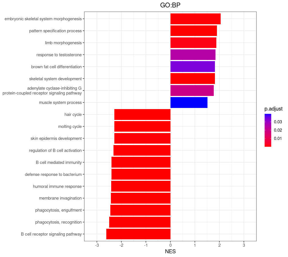
보시면 중간에 글자라 2줄로 변경된 것이 보일 겁니다.
쉽게 설명해서, NES가 음수이면 발현 감소, 양수이면 발현 증가된 pathway로 보면 됩니다.
댓글